Neural Network

Till now we learnt about Logistic Regression and Linear Regression. But in practical machine learning problems these are not enough. Let’s see why the existing algorithms are not sufficient to solve machine learning problem :

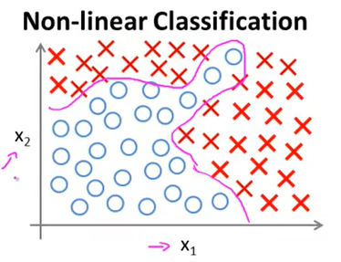
As you can see in the above classification example based on 2 features (x₁ and x₂), if we try to apply logistic regression, we will get an equation like this :

g(θ₀ + θ₁x₁ + θ₂x₂ + θ₃x₁x₂ + …)

Which is very long already. But in actual real world machine learning problem we will have roughly 100 features (or maybe more)

x₁, x₂, x₃, … x₁₀₀

Now if we try to create an equation for these many features it will be very big. For example if we just consider features of quadratic terms like (x₁x₂, x₂x₃, x₃x₅, …), the count will be ~ 5000 features. Quadratic features count roughly grows by n². So to calculate for 5000 features the values of theta will be computationally expensive and might even overfit. Now if we just include cubic features like (x₁x₂x₃, x₂x₃x₄, x₃x₅x₇, …), the count will be ~ 170000 features. This is dramatically more computationally expensive. So, that’s why existing algorithm can’t be use in most real world applications.

Another example in Computer vision. Suppose we are making an algorithm which will try to identify if an image is of a car or not. To do that assume we are just talking about 50x50 pixel images. Now these 50x50 pixel images will contain 2500 total pixels. Hence 2500 features (in just greyscale). In this scenerio if we try to take just quadratic features it will create 3 million features which is just impossible to calculate even with super computers. :(

So this is the reason we require a non linear hypothesis to work on large real world problems. Neural Netowrk is an algorithm which tries to mimic brain. It is state of the art technique for many applications.

The ‘one learning’ hypothesis

Neural networks are derived from neurons in brain. How it was developed well, there’s a theory that human intelligence stems from a single algorithm. The idea arises from experiments suggesting that the portion of your brain dedicated to processing sound from your ears could also handle sight for your eyes. This is possible only while your brain is in the earliest stages of development, but it implies that the brain is – at its core – a general-purpose machine that can be tuned to specific tasks. Now since a brain can handle multiple task why not a machine learning algorithm. So using this logic a neural network can handle any type of data as we will see later on.

Neurons

Neural networks was developed in resemblance to neurons in our brain. So to understand how a neural network works, we first need to understand how neurons in our brain work.

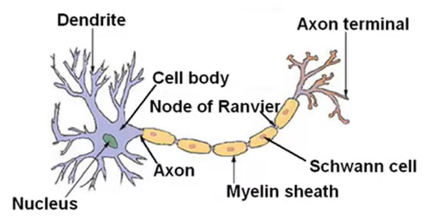
Cell body - Central computational unit
Dendrites - Input wires
Axon - Output wires

As you can see in the diagram, basically what a neuron does is that dendrite receives signal from different parts of body or other neurons. The cell body then processes that signal and axon transfers it to other neurons or muscles wherever it is connected. So it is a computational unit which takes a number of inputs does some calculations and transfers the outputs. The neurons can also communicate between each other using electric pulses. It happens when a dendrite of a neuron is connected to axon of another neuron. So second neuron can send message to first neuron.

Neuron Model

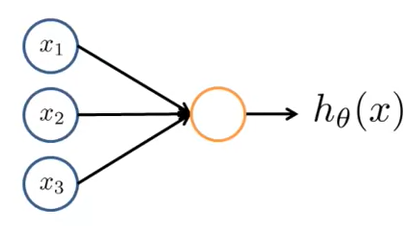
This is the simplest representation of a neuron model. Here yellow circle is where the computation happens (cell body). x₁, x₂, x₃ are Input wires or dendrites through which we get our inputs. h_θ(x) is the hypothesis which we will get after all the computation is done. It is also the axon of our neuron model. Here we will be using logistic function in computation i.e. :

h(x) = $\Large\frac{1}{1+e^{-θ^Tx}}$

Due to which this neuron model will be known as Sigmoid (logistic) activation function. Here we might sometimes draw an extra input to simplify calculations called x₀ which will always have value of 1. This extra input is called bias unit. One more important thing to note is that in our previous machine learning algorithms we denoted θ as parameters. In neural networks θ is also known as weights instead of parameters.

Neural network

The actual simplest neural network looks something like this :

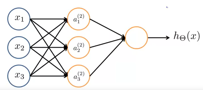
As represented in above image :

Layer 1 - Its called Input layer
Final layer - Its called Output layer
Middle layers - Activation units or Hidden layers

Here x₁, x₂, x₃ are some inputs which goes through activations functions a₁, a₂, a₃ and then again on last layer and gives some output. More formally :

x_i^(j) = “activation” of unit i in layer j
θ^(j) = Matrix of weights controlling function mapping from layer j to layer j+1

Now if you saw that we are using sigmoid function which is represented by g(z), so some computation represented by this particular neural network is :

$a_1^{(2)} = g(θ_{10}^{(1)}x_0 + θ_{11}^{(1)}x_1 + θ_{12}^{(1)}x_2 + θ_{13}^{(1)}x_3 ) $
$a_2^{(2)} = g(θ_{20}^{(1)}x_0 + θ_{21}^{(1)}x_1 + θ_{22}^{(1)}x_2 + θ_{23}^{(1)}x_3 ) $
$a_3^{(2)} = g(θ_{30}^{(1)}x_0 + θ_{31}^{(1)}x_1 + θ_{32}^{(1)}x_2 + θ_{33}^{(1)}x_3 ) $
Final function = $h_θ(x)$ = $a_1^{(3)} = g(θ_{10}^{(2)}a_0^{(2)} + θ_{11}^{(2)}a_1^{(2)} + θ_{12}^{(2)}a_2^{(2)} + θ_{13}^{(2)}a_3^{(2)} ) $

This might seems to be a lot but actually its pretty straight forward. We created this function similarly to logistic regression hypothesis function. Here :

a₁ = First hidden unit function
a₂ = Second hidden unit function
a₃ = Third hidden unit function
h = Final function

Here Each layer of neural network get’s its own set of θ. The order of θ is dependent on the inputs and activation function. So in this scenerio :

Input units = 3 Output units = 3 Order of θ⁽¹⁾ = 3 X 4 matrix

Forward Propogation : Vectorized Implementation

Now the equation’s we saw above are quite big. Let’s try to convert them into vectors. Let’s assume :

$z_1^{(2)} = θ_{10}^{(1)}x_0 + θ_{11}^{(1)}x_1 + θ_{12}^{(1)}x_2 + θ_{13}^{(1)}x_3 $
$z_2^{(2)} = θ_{20}^{(1)}x_0 + θ_{21}^{(1)}x_1 + θ_{22}^{(1)}x_2 + θ_{23}^{(1)}x_3 $
$z_3^{(2)} = θ_{30}^{(1)}x_0 + θ_{31}^{(1)}x_1 + θ_{32}^{(1)}x_2 + θ_{33}^{(1)}x_3 $

So now we got :

$a_1^{(2)} = g(z_1^{(2)})$
$a_2^{(2)} = g(z_2^{(2)})$
$a_3^{(2)} = g(z_3^{(2)})$

Now these simple equations can be converted to vectors :

x =
x₀
x₁
x₂
x₃
z⁽²⁾ =
z⁽²⁾₁
z⁽²⁾₂
z⁽²⁾₃

So in terms for vectors our equations will now be converted into :

z⁽²⁾ = θ⁽¹⁾X
$a^{(2)} = g(z^{(2)})$

Where z⁽²⁾ is a 3X1 matrix and a⁽²⁾ is 3X1 matrix. Now the inputs can also be considered as activation layers. So :

$a^{(1)} = x $
This will imply
z⁽²⁾ = θ⁽¹⁾a⁽¹⁾
In generalized term :
z^(j+1) = θ^(j)a^(j)
where j is layer number

Our hypothesis function will be :

$h_θ(x) = a^{(3)} = g(z^{(3)}) $
In generalized term :
$h_θ = a^{(j+1)} = g(z^{(j-1)})$

This process of computing h(x) is called forward propogation. It is named because we start the propogation at input units (first layer) and move forward to last layer (output).

Learning it’s own features

The biggest thing about neural network is that instead of taking original inputs through each layer to calculate it takes activation values from previous layers as depicted by diagram above. So,

Layer 1 = Input features
Layer 2 = Takes layer 1 as input (actual input)
Layer 3 = Takes layer 2 output as input (newly created features by neural network)

So, neural network learns its own features on each layer and is not contrained to original input features.

Examples

AND Function

Let’s try to create a neural network which will represent and Logic AND Function. So as far we know it will have just 2 inputs - x₁, x₂. The diagram of neural network will look like this :

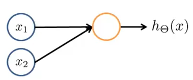
Here :

x₁, x₂ belongs to {0,1}
y belongs to x₁ AND x₂

As we learnt in previous topics and from diagram we know :

$h_θ(x)$ = $g(θ_{0}x_0 + θ_{1}x_1 + θ_{2}x_2 ) $ where x₀ = 1 (bias input)

How to find the values of θ we will see later on but let’s assume we were able to find it. So :

$θ_0$ = -30
$θ_1$ = 20
$θ_2$ = 20

After subtituting the values our equation will become :

$h_θ(x)$ = $g(-30x_0 + 20x_1 + 20x_2 ) $

We are using sigmoid activation function which is :

h(x) = g(z) = $\Large\frac{1}{1+e^{-z}}$

After putting each possible values of x₁ and x₂ we get :

x1	x2	h(x)
0	0	g(-30) = 0
0	1	g(-10) = 0
1	0	g(-10) = 0
1	1	g(10) = 1

As we can see from the table above, our neural network is able to predict and implement a Logic AND operation.

OR Function

Let’s try to create a neural network which will represent and Logic OR Function. So as far we know it will have just 2 inputs - x₁, x₂. The diagram of neural network will look like this :

Here :

x₁, x₂ belongs to {0,1}
y belongs to x₁ OR x₂

As we learnt in previous topics and from diagram we know :

$h_θ(x)$ = $ g(θ_{0}x_0 + θ_{1}x_1 + θ_{2}x_2 ) $ where x₀ = 1 (bias input)

How to find the values of θ we will see later on but let’s assume we were able to find it. So :

$θ_0$ = -10
$θ_1$ = 20
$θ_2$ = 20

After subtituting the values our equation will become :

$h_θ(x)$ = $ g(-10x_0 + 20x_1 + 20x_2 ) $

We are using sigmoid activation function which is :

h(x) = g(z) = $\Large\frac{1}{1+e^{-z}}$

After putting each possible values of x₁ and x₂ we get :

x1	x2	h(x)
0	0	g(-10) = 0
0	1	g(10) = 1
1	0	g(10) = 1
1	1	g(30) = 1

As we can see from the table above, our neural network is able to predict and implement a Logic OR operation.

NOT Function

Let’s try to create a neural network which will represent and Logic NOT Function. So as far we know it will have just 1 input - x₁. The diagram of neural network will look like this :

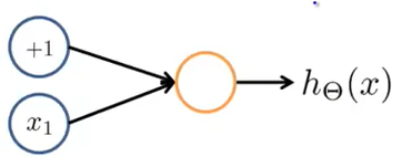
Here :

x₁ belongs to {0,1}
y belongs to NOT of x₁

As we learnt in previous topics and from diagram we know :

$h_θ(x)$ = $ g(θ_{0}x_0 + θ_{1}x_1 ) $ where x₀ = 1 (bias input)

How to find the values of θ we will see later on but let’s assume we were able to find it. So :

$θ_0$ = 10
$θ_1$ = -20

After subtituting the values our equation will become :

$h_θ(x)$ = $ g(10x_0 - 20x_1 ) $

We are using sigmoid activation function which is :

h(x) = g(z) = $\Large\frac{1}{1+e^{-z}}$

After putting each possible values of x₁ and x₂ we get :

x1	h(x)
0	g(10) = 1
1	g(-10) = 0

As we can see from the table above, our neural network is able to predict and implement a Logic NOT operation.

XNOR Function

Let’s try to create a neural network which will represent and Logic XNOR Function. Instead of creating new neural network we will try to use the 3 existing neural network and club them. Let’s see this new neural network :

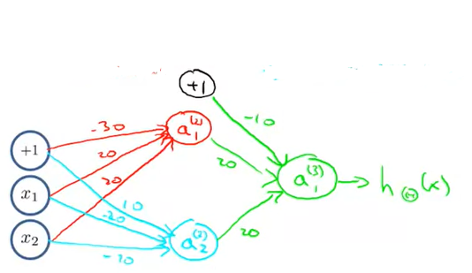
Here red represents AND Neural network, Blue represents Not x and Not x and green represents OR neural network. All the values of θ are shown in the image. So after substituting we will get :

x1	x2	a1	a2	h(x)
0	0	0	1	1
0	1	0	0	0
1	0	0	0	0
1	1	1	0	1

As we can see from the table above, our neural network is able to predict and implement a Logic XNOR operation. This was an example with 2 layer of neural network. Similarly we can create any number of layers.

MultiClass Classification

Till now we were working when the output was of range either 0 or 1. But what if our output is of range 0,1,2,3,4 etc? For eg :

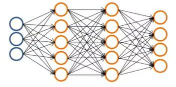
As you can see in the above image the final layer has 4 h(x). So in this scenerio instead of getting h(x) = 0,1,2,3 we will get a vector of values of h(x). So if h(x) vector contained :

0
0
1
0

The 3rd value is 1 so our neural network will select the 3rd category as output. That is how our multiclass neural network works.