Multivariate Linear Regression

This is quite similar to the simple linear regression model we have discussed previously, but with multiple independent variables contributing to the dependent variable and hence multiple coefficients to determine and complex computation due to the added variables. Till now we were only using 1 input feature. Like in our House price prediction example we were trying to predict price of the house just on the size of house. But in practical this is not the only factor on which price of house depends. Their are various other factors like Number of bedrooms, number of floors, age of house etc.

Updated House Price Problem

Suppose your friend is selling his/her house, and you want to create a model which will predict the price of the house so that your friend don’t incur a loss. So for you to create a model you will first need to collect details for houses in your friends locality.

Size (x1)	No of bedrooms (x2)	No of floors (x3)	Age of home (x4)	Price (y)
2104	5	1	45	460
1416	3	2	40	232
1534	3	2	30	315
852	2	1	36	178
…	…	…	…	…

Some of the notation which will be used through out -

m = Total number of data sets n = Number of features x⁽ⁱ⁾ = Input feature of i^th example x⁽ⁱ⁾_j = Value of feature j in i^th training example y = Output variable or Target

Some example :

x² = 1416, 3, 2, 40
x²₃ = 2

---

Hypothesis Function

Previously with just 1 feature our hypothesis function looked like :

h(x) = θ₀ + θ₁x

But now with introduction of multiple features, our function will look like :

h(x) = θ₀ + θ₁x₁ + θ₂x₂ + θ₃x₃ + θ₄x₄

An example what this new hypothesis function look like if we substitute θ :

h(x) = 80 + 0.1x₁ + 0.01x₂ + 3x₃ - 2x₄

NOTE - Here +ve coefficient denotes that that feature increases the price of house and a -ve coefficient denotes that that feature decreases the price of house.

Now if we try to generalize the hypothesis function for n input feature, it would look something like this :

h(x) = θ₀ + θ₁x₁ + θ₂x₂ + …. + θ_nx_n

For ease of understanding we can even convert the above equation into a matrix form. How ? First for convenience of notation let us define :

x₀ = 1

Now our generalized hypothesis equation can be written as :

h(x) = θ₀x₀ + θ₁x₁ + θ₂x₂ + …. + θ_nx_n

Secondly lets define 2 matrices :

x
x₀
x₁
x₂
:
:
x_n
θ
θ₀
θ₁
:
:
θ_n

Now using matrix matrix multiplication method our generalized hypothesis function can be written as :

h(x) = θ^Tx

The above equation is very simple matrix form of our general hypothesis function.

Gradient Descent

Gradient descent is a first-order iterative optimization algorithm for finding a local minimum of a differentiable function. The idea is to take repeated steps in the opposite direction of the gradient (or approximate gradient) of the function at the current point, because this is the direction of steepest descent. So this is an algo to find minimum of any function. So here we want :

min (J(θ₀ , θ₁, …, θ_n))

So our algorithm will become :
Repeat until convergence {

θ_j = θ_j - $\alpha$ $\Large\frac{d}{dθ_j}$ J(θ₀ , θ₁, …, θ_n)
}

Here, θ₀, θ₁, …, θ_n needs to be updated simultaneously. Now putting our cost function and actual differential calculus we wont be covering here. So let’s directly jump to the outcome after applying the differentiation on our gradient descent algorithm :
Repeat until convergence {

θ_j = θ_j - $\alpha$ $\Large\frac{1}{m}$ $\sum_{i=1}^m (h_\theta(x^{(i)}) - y^{(i)}).x_j^{(i)}$
}

Here simultaneously update θ_j for j=0,1,…n, Where x₀⁽ⁱ⁾ = 1 as assumed previously.

---

Making Gradient Descent Faster

We can speed up gradient descent by having each of our input values in roughly the same range. This is because θ will descend quickly on small ranges and slowly on large ranges, and so will oscillate inefficiently down to the optimum when the variables are very uneven. The way to prevent this is to modify the ranges of our input variables so that they are all roughly the same. Ideally :

−1 ≤ $x_{(i)}$ ≤ 1 or −0.5 ≤ $x_{(i)}$ ≤ 0.5

These aren’t exact requirements; we are only trying to speed things up. The goal is to get all input variables into roughly one of these ranges, give or take a few. Now let’s see what will happen if the scale of features are very different. Like :

x₁ = Size of house (0-2000 feet)
x₂ = Number of bedrooms (1-5)

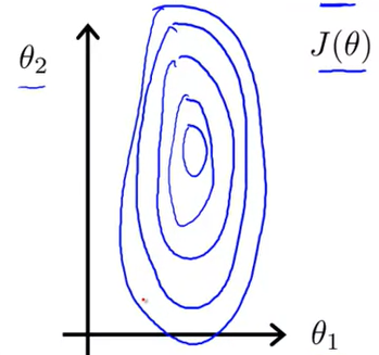
If we try to plot it, it will look something like this :

Now as you can see, It will be very elliptical curve and hence it will take a very long time to reach global minimum. Now for making features scale to same level their are 2 ways to do it.

Feature Scaling

Feature scaling involves dividing the input values by the range (i.e. the maximum value minus the minimum value) of the input variable, resulting in a new range of just 1. In this scenerio we can make the scaling more equal by :

x₁ = $\Large\frac{value}{range}$

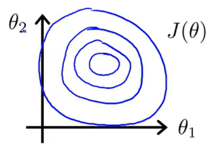
By this method our feature will be in range of −1 ≤ $x_{(i)}$ ≤ 1 or atleast close enough. If we try to plot it, it will look something like this :

Now as you can see, It will be a circular curve and hence It will take very less time/iterations to reach global minimum.

Mean Normalization

Mean normalization involves subtracting the average value for an input variable from the values for that input variable resulting in a new average value for the input variable of just zero. In this scenerio we can make scaling more equal by :

x₁ = $\Large\frac{x_i-μ_i}{s_i}$

Where :

x_i = Feature
μ_i = Mean of feature
s_i = Range of feature

For example, if x_i represents housing prices with a range of 100 to 2000 and a mean value of 1000, then, x_i = $\Large\frac{price-1000}{1900}$.

Gradient Descent : Correctly Working?

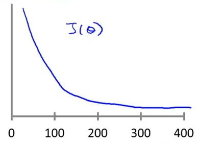
Their is a way to check if gradient descent algorithm is working correctly or not for the given cost function. To do that we need to plot a grpah with the number of iteration of gradient descent versus the cost function values. If we plot them it will look something like this :

Now if your graph is continously decreasing that means your gradient descent algorithm is working correctly and no changes is required. But if your graph is increasing or is a zig-zag graph that means learning rate of your algorithm needs to be changed. Some pointers :

1. If your graph is increasing then learning rate needs to be decreased.
2. If your graph is in a zig-zag format then learning rate needs to be decreased.
3. If learning rate is too small, gradient descent will be slow to convergence.
4. If learning rate is large, gradient descent may not decrease and thus may not converge.

Creating new features

We can even create new features from given feature. Suppose in our house prediction problem if we were given frontage and depth our hypothesis function would have been looked like :

h(x) = θ₀ + θ₁xFrontage + θ₂xDepth

Now we can create a new feature something called - “area”. Where :

area = Frontage X Deapth

So now our hypothesis function will look like :

h(x) = θ₀ + θ₁xArea

Polynomial Regression

Sometimes, Linear models doesn’t fit well with our data and in that scenerio we can try some polynomial regression. Here our hypothesis function will look like :

h(x) = θ₀ + θ₁X + θ₂X²
h(x) = θ₀ + θ₁X + θ₂X² + θ₃X³

More details we will see later. But one thing to keep in mind that in polynomial regression, feature scaling is very important.