Logistic Regression

The logistic model (or logit model) is used to model the probability of a certain class or event existing such as pass/fail, win/lose, alive/dead or healthy/sick. Now lets try to find values of θ for our hypothesis function. But before that let’s first layout our initial things. Suppose we have a training set :

{(x¹, y¹), (x², y²), (x³, y³), …, (x^m, y^m)}
Total m examples
y belongs in {0,1}

Our hypothesis function

h(x) = $\Large\frac{1}{1+e^{-θ^Tx}}$

Now our biggest question is how do we choose values for θ.

How to choose θ?

Now if we remember our previous sections of linear regression, we used squared error cost function. Which was :

J(θ) = $\Large\frac{1}{2m}$ $\sum_{i=1}^m (h_\theta(x^{(i)}) - y^{(i)})^2 $

Now this method to find the cost worked perfectly for linear regression as it made convex function (A function which has 1 global minimum). But here if we try to apply the cost to our hypothesis function of logistic regression it will create a non-convex function (A function which has many local minimum) and due to which we will not be able to find minimum values of θ properly. So to make it work we have to come up with another solution. To do it, let’s define a new cost function :

{ -log(h_θ(x)) if y = 1 }
{ -log(1 - h_θ(x)) if y = 0 }

Let’s analyze it :

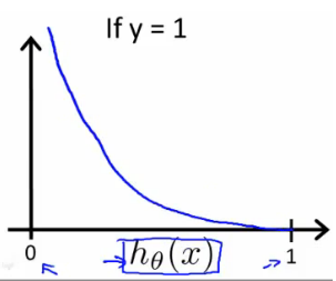
As you can see in the above plot, this is plot of logistic regression/hypothesis function if we take y=1. It has below advantages :

1. If y=1 & it predicts h(x)=1 then Cost=0, as you can analyze through the plot
2. If y=1 & it predicts h(x)=0 then Cost=∞ So the basic is that if our algo predicts wrongly the algorithm is heavily penalized.

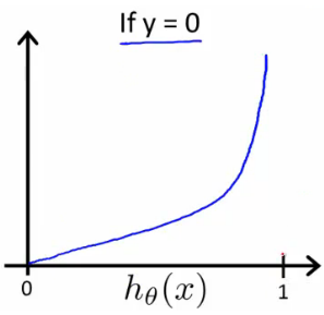
As you can see in the above plot, this is plot of logistic regression/hypothesis function if we take y=0. It has below advantages :

1. If y=0 & it predicts h(x)=0 then Cost=0, as you can analyze through the plot
2. If y=0 & it predicts h(x)=1 then Cost=∞ So the basic is that if our algo predicts wrongly the algorithm is heavily penalized. Our new cost function is working as expected till now. But still this cost function looks little complex. Let’s try to simplify it.

Simplified Cost Function

As we saw in previous section our new cost function looks something like this :

{ -log(h_θ(x)) if y = 1 }
{ -log(1 - h_θ(x)) if y = 0 }

But it looks a lot complex, Let’s try to combine it within a single line/single equation. So,

Cost(h_θ(x), y) = - ylog(h_θ(x)) - (1 - y)log(1 - h_θ(x))

But is this new equation correct? Let’s check it once :

If y = 0 then Cost(h_θ(x), y) = -log(h_θ(x))
If y = 1 then Cost(h_θ(x), y) = -log(1 - h_θ(x))

So it works correctly. Now this function is for just 1 training data. We need to generalize it for all m training data. So our new Cost function will become :

J(θ) = - $\Large\frac{1}{m}$ $\sum_{i=1}^m ( ylogh_\theta(x) + (1 - y)log(1 - h_\theta(x)))$

So now we got our cost function, we just have to find values of θ which will minimize J(θ). And what is better to minimize then our own Gradient Descent.

Gradient Descent Algorithm

If you remember from past sections Gradient Descent algorithm looks like this :

Repeat until convergence {

θ_j = θ_j - $\alpha$ $\Large\frac{d}{dθ_j}$ J(θ)
}

After substituting the new value of J(θ) and taking derivative (again we wont go into details of actual derivation) it will become :

θ_j = θ_j - $\alpha$ $\sum_{i=1}^m (h_\theta(x^{(i)}) - y^{(i)}).x^{(i)}$

Do you remember the above equation from somewhere? It was exactly the same equation which we used in Linear Regression. So, even if our cost function are different the gradient descent is same for both Logistic Regression and Linear regression. One thing to remember even if gradient descent is same it doesnt mean both algorithm are same. Because in one algo we are predicting the values using sigmoid function and in another we are predicting the values using linear algebra. So both are not same. Since we have used gradient descent here that means all properties of it are followed here.

Advanced Optimizations

From starting of this course we are just talking about only 1 algorithm to find minimum of a function i.e. Gradient Descent. But their are other algorithms as well :

1. Conjugate gradient
2. BFGS
3. L-BFGS

Now we won’t go into detail of how these 3 algorithms work. But they have some advantages and disadvantages over gradient descent :

1. In these you dont need to manually pick $\alpha$
2. These are faster than gradient descent
3. These are more complex to implement and understand than gradient descent

Multiclass Classification

In machine learning, multiclass or multinomial classification is the problem of classifying instances into one of three or more classes. A classification task with more than two classes; e.g., classify a set of images of fruits which may be oranges, apples, or pears. Multi-class classification makes the assumption that each sample is assigned to one and only one label: a fruit can be either an apple or a pear but not both at the same time. Till now we are working on binary classification i.e. where output can be only 1 out of 2 values. But we might get scenerio where we need to predict 1 out of 3 or more options. This is called Multiclass Classification. Examples :

1. Sorting of e-mail into - Work, Friend, Family and Hobby category.
2. Medical diagnosis of flu into - Not ill, cold or Flu.
3. Weather Prediction into - Sunny, Cloudy, Rain or Snow

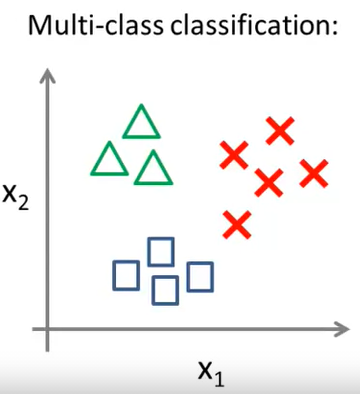
Now let’s see how exactly it will look like in graph :

Here the objects are from 3 categories - Square, triangle and cross. So for any new object we will require to predict if that object will be a square, triangle or a cross. So here our y will be of :

y = {0, 1, 2}

To do that we will use something called One-vs-all theory.

One-Vs-All

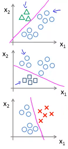
In one-vs-All classification, for the N-class instances dataset, we have to generate the N-binary classifier models. The number of class labels present in the dataset and the number of generated binary classifiers must be the same. So in simple words, our logistic regression algorithm was based on binary classification. So we now need to divide our multiclass classification into binary classification. So N-Multiclass classification problem will be converted to N-binary classification problem. In our above example it will be converted into 3 parts :

Each for y = {0, 1, 2}

So as seen in the above image we created 3 binary classifier for our multiclass problem :

Classifier 1:- Green vs [Red, Blue]
Classifier 2:- Blue vs [Green, Red]
Classifier 3:- Red vs [Blue, Green]

Part 1

So here we are assuming that we are trying to predict class is Green and rest all are converted into a random different class (like here as circle). So now we create a hypothesis function h¹(x) for this case which will predict if it is a Green or not.

Part 2

So here we are assuming that we are trying to predict class is Blue and rest all are converted into a random different class (like here as circle). So now we create a hypothesis function h²(x) for this case which will predict if it is a Blue or not.

Part 3

So here we are assuming that we are trying to predict class is Red and rest all are converted into a random different class (like here as circle). So now we create a hypothesis function h³(x) for this case which will predict if it is a Red or not.

After calculating all these h(x) values we will select the class for which h(x) will be maximum.

So now our algorithm will become :

Train a logistic regression classifier hⁱ(x) for each class i to predict the probability that y=i
On a new input x, to make a prediction, pick the class i that maximizes hⁱ(x)