What is Linear Regression with one variable?

Linear Regression is a machine learning algorithm based on supervised learning. It performs a regression task. Regression models a target prediction value based on independent variables. It is mostly used for finding out the relationship between variables and forecasting. Different regression models differ based on – the kind of relationship between dependent and independent variables, they are considering and the number of independent variables being used.

Linear regression performs the task to predict a dependent variable value (y) based on a given independent variable (x). So, this regression technique finds out a linear relationship between x (input) and y(output). Hence, the name is Linear Regression.

Sounds tough? Lets analyze with an example.

House Price Problem

Suppose your friend is selling his/her house, and you want to create a model which will predict the price of the house so that your friend don’t incur a loss. So for you to create a model you will first need to collect details for houses in your friends locality. As of now we will assume only size of the house is enough (but in real world its not) to predict the price.

Size (x)	Price (y)
2104	460
1416	232
1534	460
…	…
…	…

You will most likely collect data in the above format. But does that give you any usefull info at the moment? No. Let’s look at this data in a different way. Let’s plot the above data into a graph with size being the X-Axis and price being in Y-Axis.

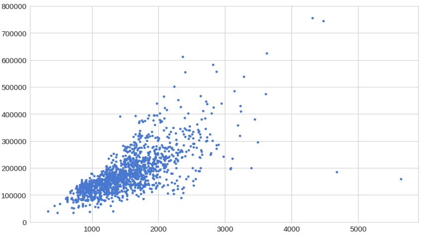
Now are you able to see any pattern in the data?

So, if we try to fit a straight line across these points, it’s called Linear Regression.

Since we have only 1 X variable it is called linear regression with 1 variable.

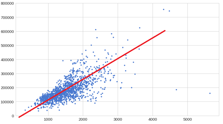
Now this data set (data which we have collected) is also called Training set.

Some of the notation which will be used through out -

m = Total number of data sets
x = Input variable or Feature
y = Output variable or Target
(x,y) = Any training set example

---

How ML model is created?

The training set (data) is fed to a learning algorithm which creates a h function also called hypothesis function. This function take X as input and gives Y as output.

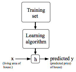
So for our example the machine learning algorithm will create an h function (hypothesis function) which will take size as input and will provide prediction of cost of the house as output.

It will be denoted as -

h(x) = θ₀ + θ₁x

In mathematical notation -

h : x -> y

Now, our task is to find the value of θ₀ and θ₁

---

Cost function

Let’s assume some values of θ₀ and θ₁

Below we tried to guess the values of θ₀ and θ₁ and plotted them onto the X and Y axis

But still we need to determine what will be the perfect value for θ₀ and θ₁

The perfect value of θ₀ and θ₁ is that which will make h(x) as close as possible to y.

In simpler terms :

The difference betwwen the derived ‘y’ and the actual ‘y’ should be minimum.

In mathematical terms :

Minimize -> $\Large\frac{1}{2m}$ $\sum_{i=1}^m (h_\theta(x^{(i)}) - y^{(i)})^2 $

where $h_\theta(x^{(i)}) = \theta_0 + \theta_1x^{(i)}$

The above equation is called Cost Function which is denoted by - J(θ₀, θ₁)

This mathematical notation is also called Squared Error Function or Mean Squared Error which is commonly used in regression problems.

Too much mathematics? Let’s simplify it.

Simplified Cost function

Let’s assume θ₀ = 0

$h_\theta(x) = \theta_1x$
$J(\theta_1) = \Large\frac{1}{2m}$ $\sum_{i=1}^m (h_\theta(x^{(i)}) - y^{(i)})^2 $

Case 1 :

Let’s assume θ₁ = 1

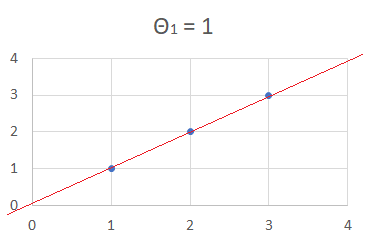
$h_\theta(x) = x$
$J(\theta_1) = \Large\frac{1}{2m}$ $\sum_{i=1}^m (h_\theta(x^{(i)}) - y^{(i)})^2 $
$J(1) = \Large\frac{1}{2\times3}$ $((1 - 1)^2 + (2 - 2)^2 + (3 - 3)^2)$
$J(1) = 0$

Case 2 :

Let’s assume θ₁ = 0.5

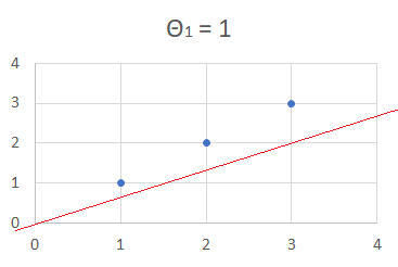
$h_\theta(x) = 0.5x$
$J(\theta_1) = \Large\frac{1}{2m}$ $\sum_{i=1}^m (h_\theta(x^{(i)}) - y^{(i)})^2 $
$J(0.5) = \Large\frac{1}{2\times3}$ $((0.5 - 1)^2 + (1 - 2)^2 + (1.5 - 3)^2)$
$J(0.5) = \Large\frac{3.5}{6}$
$J(0.5) = 0.58$

Case 3 :

Let’s assume θ₁ = 0

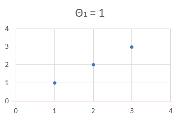
$h_\theta(x) = 0$
$J(\theta_1) = \Large\frac{1}{2m}$ $\sum_{i=1}^m (h_\theta(x^{(i)}) - y^{(i)})^2 $
$J(0) = \Large\frac{1}{2\times3}$ $((0 - 1)^2 + (0 - 2)^2 + (0 - 3)^2)$
$J(0) = \Large\frac{14}{6}$
$J(0) = 2.33$

Now we got different values of cost function due to different values of θ. But which one makes the cost function minimum? For simplicity lets plot these values in a graph.

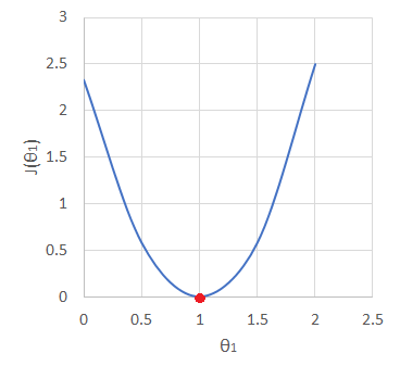
So after plotting we are able to identify when cost function reaches it’s minimum value for corresponding θ value. Hence our machine learning has achieved maximum accuracy.

Coming back

Coming back to our scenerio when we need to find the values of both θ₀ and θ₁. If we go by above method we will get a 3-D graph. We cant plot a 3 variable graph on a 2-D plane but it will look something like this

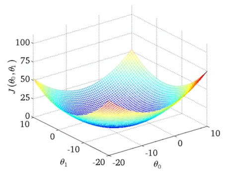
Now as the features will increase plotting them on a 2-D plane will become impossible. So to overcome this fault we will be using contour plots. Which will look like this

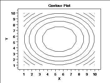
We will require to reach middle part of this, and to make things easy their is already an algorithm to find minimum and reach it.