Gradient Descent

Gradient descent is a first-order iterative optimization algorithm for finding a local minimum of a differentiable function. The idea is to take repeated steps in the opposite direction of the gradient (or approximate gradient) of the function at the current point, because this is the direction of steepest descent. So this is an algo to find minimum of any function. In our case J(θ₀ , θ₁). So here we want :

min (J(θ₀ , θ₁))

Outline

1. Start with some θ₀ and θ₁. ( Say example - θ₀ = 0 , θ₁ = 0 )
2. Keep changing θ₀ and θ₁ to reduce J(θ₀ , θ₁) until we hopefully end up at a minimum.

So basically, suppose at first run of the gradient descent we started at x₁. We will move in a direction in which our function is becoming minimum. Hence we will arrive at y₁. If we run gradient descent again, we would have started either at x₂ or x₃ and hence we would have reached at either y₂ or y₃. So, it gives us local minimum depending upon where we are starting in each turn.

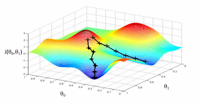
Gradient Descent Algorithm

Repeat until convergence {

θ_j = θ_j - $\alpha$ $\Large\frac{d}{dθ_j}$ J(θ₀ , θ₁)
}

Here, θ₀ & θ₁ needs to be updated simultaneously. So,

temp0 = θ₀ - $\alpha$ $\Large\frac{d}{dθ_0}$ J(θ₀ , θ₁)
temp1 = θ₁ - $\alpha$ $\Large\frac{d}{dθ_1}$ J(θ₀ , θ₁)
θ₀ = temp0
θ₁ = temp1

Here, $\alpha$ is called learning rate. It controls how big a step we are taking to move towards convergence. In simplest terms $\Large\frac{d}{dθ_0}$ J(θ₀ , θ₁) is slope of a tangent on graph point θ₀ , θ₁ .

Gradient Descent for single parameter

Here we are only considering θ₁. So gradient descent algorithm will become : Repeat until convergence {

θ₁ = θ₁ - $\alpha$ $\Large\frac{d}{dθ_1}$ J(θ₁)
}

Now lets analyze how the algorithm will run.

Case 1 :

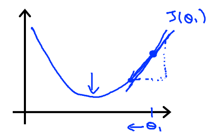
As seen in the image let’s assume we started at the given point. Now we drew a tangent to the point. Now the slope if we calculate it will come a positive integer. So,

$\Large\frac{d}{dθ_1}$ J(θ₁) >= 0
θ₁ = θ₁ - $\alpha$(+ number)

Now if we repeat the algorithm θ₁ will decrease and we will reach local minimum.

Case 2 :

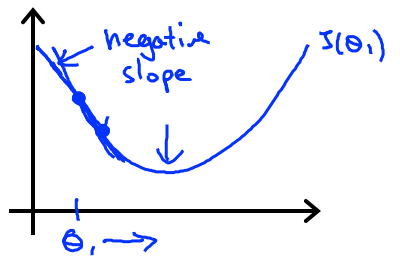
As seen in the image let’s assume we started at the given point. Now we drew a tangent to the point. Now the slope if we calculate it will come a negative integer. So,

$\Large\frac{d}{dθ_1}$ J(θ₁) <= 0
θ₁ = θ₁ - $\alpha$(- number)

Now if we repeat the algorithm θ₁ will increase and we will reach local minimum.

Learning Rate

1. If $\alpha$ is too small, gradient descent will be too slow as it will take small steps to proceed.
2. If $\alpha$ is too large, gradient descent can overshoot the minimum. It may fail to converge or even diverge.

Gradient Descent at local minimum

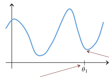
As seen in the image let’s assume we started at the given point. Now we drew a tangent to the point. This tangent will be parellel to the x-axis. Hence making the slope be 0. So :

$\Large\frac{d}{dθ_1}$ J(θ₁) = 0
θ₁ = θ₁ - $\alpha$(0)

So it will leave θ₁ unchanged. The algorithm will stop as expected.

Gradient Descent to our cost function

Now lets apply the gradient descent algorithm to the cost function of linear regression which we studied in last topic. So if we recall :

h(x) = θ₀ + θ₁x
J(θ₀ , θ₁) = $\Large\frac{1}{2m}$ $\sum_{i=1}^m (h_\theta(x^{(i)}) - y^{(i)})^2 $

Now actual differential calculus we wont be covering here. So let’s directly jump to the outcome after applying the differentiation.

θ₀ = $\Large\frac{1}{m}$ $\sum_{i=1}^m (h_\theta(x^{(i)}) - y^{(i)})$
θ₁ = $\Large\frac{1}{m}$ $\sum_{i=1}^m (h_\theta(x^{(i)}) - y^{(i)}).x^{(i)}$

After all the mathematical calculations, we can apply the below Gradient descent algorithm to our linear regression cost function :
Repeat until convergence {

θ₀ = θ₀ - $\alpha$ $\Large\frac{1}{m}$ $\sum_{i=1}^m (h_\theta(x^{(i)}) - y^{(i)})$
θ₁ = θ₁ - $\alpha$ $\Large\frac{1}{m}$ $\sum_{i=1}^m (h_\theta(x^{(i)}) - y^{(i)}).x^{(i)}$ }

And now we have successfully understood the gradient descent algorithm as well as applied it to our linear regression cost function.

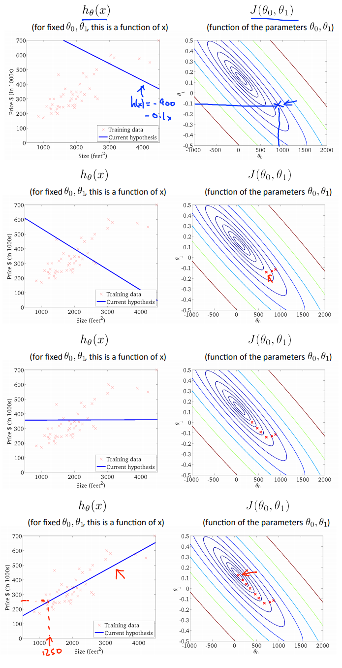
As you can see in the above image, we applied gradient descent algo and we came to a point where our machine learning algorithm will be able to predict the house prices closely as possible.

Note :

1. The graph of linear regression is a bowl-shaped graph. It is called Convex function. It doesnt have local optima but only 1 global optimum. So what it means that no matter at which point we start our gradient descent algorithm we will always reach the global minimum of the function.
2. This approach of gradient descent is also called batch gradient descent as it uses all the training example for each iteration. So mathematically, it is a little bit slower.