Cost Function

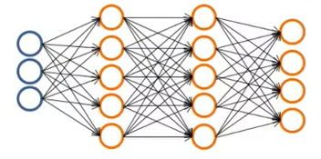
In previous section we talked about using neural network to create a Logical AND, OR, and XNOR gate. In those examples we assumed the values of θ. But how do we actually calculate them? To do that first we need to define cost function of neural network. To do that lets see a neural network :

Let’s define some terminologies :

L = Total number of layers in network
S_l = Number of units (not counting bias unit) in layer l
K = Number of output units/classes

So in our above example L = 4 and S₄ = 4. Now for binary classification :

S_L = 1
k = 1

For multiclass classification

S_L = k
k >= 3

Recall that in neural networks, we may have many output nodes. We denote $h_θ(x)$_k as being a hypothesis that results in the $k^{th}$ output. Our cost function for neural networks is going to be a generalization of the one we used for logistic regression. Recall that the cost function for regularized logistic regression was :

J(θ) = - $\Large\frac{1}{m}$ $\sum_{i=1}^m ( ylogh_\theta(x) + (1 - y)log(1 - h_\theta(x)))$ + $\frac{\lambda}{2m}\sum_{j=1}^{m}\theta_j^2$

For neural networks, it is going to be slightly more complicated :

J(θ) = - $\Large\frac{1}{m}$ $\sum_{i=1}^m\sum_{k=1}^K ( y_k^{(i)}logh_\theta(x^{(i)})$_k + $(1 - y^{(i)}$_k$)log(1 - h_\theta(x^{(i)})$_k$))$ + $\frac{\lambda}{2m}\sum_{l=1}^{L-1}\sum_{i=1}^{S_l}\sum_{j=1}^{S_{l+1}}(\theta_{ji}^{(l)})^2$

We have added a few nested summations to account for our multiple output nodes. In the first part of the equation, before the square brackets, we have an additional nested summation that loops through the number of output nodes. In the regularization part, after the square brackets, we must account for multiple theta matrices. The number of columns in our current theta matrix is equal to the number of nodes in our current layer (including the bias unit). The number of rows in our current theta matrix is equal to the number of nodes in the next layer (excluding the bias unit). As before with logistic regression, we square every term.

Note :

1. The double sum simply adds up the logistic regression costs calculated for each cell in the output layer
2. The triple sum simply adds up the squares of all the individual Θs in the entire network.
3. The i in the triple sum does not refer to training example i

Backpropagation

So, in previous topic we learnt the cost function of neural network. No we need to minimize it. “Backpropagation” is neural-network terminology for minimizing our cost function, just like what we were doing with gradient descent in logistic and linear regression. Our goal is to compute :

min J(θ)

That is, we want to minimize our cost function J using an optimal set of parameters in theta. In this section we’ll look at the equations we use to compute the partial derivative of J(Θ) :

$\Large\frac{d}{dθ_{ij}^{(l)}}$ J(Θ)

To this let’s consider the scenerio when we have just 1 training example (x,y), and we have a neural network like this :

So first we calculate forward propagation with some random value of θ :

a⁽¹⁾ = x
z⁽²⁾ = θ⁽¹⁾a⁽¹⁾
a⁽²⁾ = g(z⁽²⁾)
z⁽³⁾ = θ⁽²⁾a⁽²⁾
a⁽³⁾ = g(z⁽³⁾)
z⁽⁴⁾ = θ⁽³⁾a⁽³⁾
a⁽⁴⁾ = h_θ(x) = g(z⁽⁴⁾)

Now we calculate

$\delta_j^{(l)}$ = “Error” of node j in layer l

We start from last layer as we know what output it will be :

$\delta_j^{(4)}$ = $a_j^{(4)} - y_j$ Difference between hypothesis output and actual output
$\delta_j^{(4)}$ = $(h_θ^{(x)})$_j - $y_j$

Now we compute delta for earlier terms

$\delta_j^{(3)}$ = $(θ^{(3)})^T\delta^{4} .* a^{(3)} .* (1 - a^{(3)})$
$\delta_j^{(2)}$ = $(θ^{(2)})^T\delta^{3} .* a^{(2)} .* (1 - a^{(2)})$

Back propogation term is coined because we start at last layer and work our way backward to reduce the error.

Algorithm

• Training set {$(x^{(1)}, y^{(1)}), … , (x^{(m)}, y^{(m)})$}
  
• Set $\Delta_{ij}^{(l)} = 0$ for all i,j,l
• for i=1 to m :
  • set $a^{(1)} = x^{(i)}$
  • Perform forward propagation to compute $a^{(l)}$ for all l=2,3,…L
  • Using $y^{(i)}$ compute $\delta^{(L)} = a^{(L)} - y^{(i)}$
  • Compute $\delta^{(L-1)}, \delta^{(L-2)}, … , \delta^{(2)}$
  • $\Delta_{ij}^{(l)} := \Delta_{ij}^{(l)} + a_j^{(l)}\delta_i^{(l+1)}$
• $D_{ij}^{(l)} := $ $\Large\frac{1}{m}$$\Delta_{ij}^{(l)} + \lambdaθ_{ij}^{(l)} $if j is not equal to 0
• $D_{ij}^{(l)} := $ $\Large\frac{1}{m}$$\Delta_{ij}^{(l)} $ if j is equal to 0