Classification problems

In machine learning, classification refers to a predictive modeling problem where a class label is predicted for a given example of input data. Examples of classification problems include:

1. Given an example, classify if it is spam or not.
2. Given a handwritten character, classify it as one of the known characters.
3. Given recent user behavior, classify as churn or not.

From a modeling perspective, classification requires a training dataset with many examples of inputs and outputs from which to learn.A model will use the training dataset and will calculate how to best map examples of input data to specific class labels. As such, the training dataset must be sufficiently representative of the problem and have many examples of each class label. Class labels are often string values, e.g. “spam,” “not spam,” and must be mapped to numeric values before being provided to an algorithm for modeling.

Tumor Prediction Problem

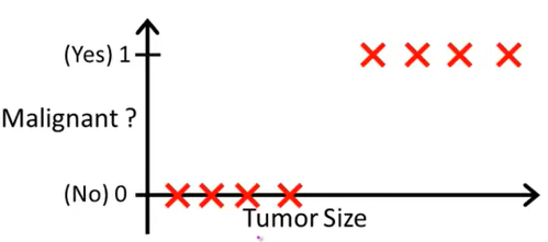
Suppose we want to create a model which will predict if a tumor is malignant or benign. So for you to create a model you will first need to collect details for the tumor. As of now we will assume only size of the tumor is enough (but in real world its not) to predict if its malignant or benign.

So in the above graph we can draw X-axis as tumor size and Y-axis as 2 outputs :

0 : Tumor is benign
1 : Tumor is malignant

Now we can try to fit linear regression algorithm in this classification problem. So we will have :

h(x) = θ^TX

Our prediction should be of only 2 outputs i.e either 1 or 0 but linear regression gives output as a Real number. So we can try to put threshold classifier at (let’s say) 0.5 :

if h(x) >= 0.5, predict “y=1”
if h(x) < 0.5, predict “y=0”

But linear regression doesn’t work properly in the cases of classification as when we work on a real word problem, at that moment no straight line can be fit in our data. So if it is working in your case then you might be lucky :) . One more issue is their with linear regression that h(x) value can be less than 0 and greater than 1 even but we want only values either 0 or 1. So it becomes tough to create a demarcation of what to take as 0 and 1.

Hypothesis Function

Now let’s try to solve the above problem using machine learning concept. So firstly we require a hypothesis function which should be :

0 <= h(x) <=1 Since we expect an output of either 0 or 1

If you remember from previous sections, hypothesis function in linear regression was :

h(x) = θ^TX

But as we seen in above topic this hypothesis function doesnt properly work in case of classification problem. To solve it let’s define a new function :

h(x) = g(θ^TX)
where g(z) = $\Large\frac{1}{1+e^{-z}}$

This newly defined g(z) function is also called sigmoid / logistic function. So, our hypothesis function will become :

h(x) = $\Large\frac{1}{1+e^{-θ^Tx}}$

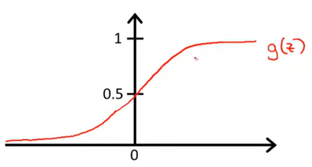
If we try to plot this function it will look something like this :

Why we converted our existing hypothesis function to a logistic function? Well the answer lies in the above graph. As you can see the output of this function always lies between 0 and 1, which we want our hypothesis function to return. Hence our original condition is satisfied by this new function. So we now simply need to find the values of θ and after putting them we can start predicting the result.

Interpretation of Hypothesis Function

In previous section we saw that h(x) returns a value between 0 and 1. So how exactly is it useful since we are interested in only 0 and 1? To understand that think about hypothesis function with respect to probability. How ? :

h(x) = estimated probability that y=1 on input x

What does it mean? Suppose we are trying to predict if a tumor is benign or malignant. So we input the tumor size for which we are predicting into the hypothesis function. Let’s say the hypothesis function returned and output 0.7. So what it actually means is that their is a 70% chance of tumor being malignant. So,

h(x) = P(y=1|x;θ)
Probability that y=1, given x, parameterized by θ
Similarly h(x) = 1 - P(y=0|x;θ)

The last line is based on probability that P_b = 1 - P_a. Since we want an answer in the form of 0 or 1, we can have :

if h(x) >= 0.5 - Predict y=1
if h(x) < 0.5 - Predict y=0

Decision Boundary

Can you see any similarity in the plot for the sigmoid function ? Well if you see clearly it provides us with 2 things :

1. g(z) >= 0.5 when z >= 0
2. g(z) < 0.5 when z < 0

If we subtitute this value in our hypothesis function we can reach to a very easy subtitution that is :

1. Whenever θ^TX >= 0 it implies h(x) >= 0.5 and we can predict y = 1
2. Whenever θ^TX < 0 it implies h(x) < 0.5 and we can predict y = 0

So we got to know that instead of finding exact value of h(x), if we just got to know that if θ^TX is less than or greater than 0 then we can easily predict y either 0 or 1. Now let’s see it with an example. Let’s assume our hypothesis function looks like :

h(x) = g(θ₀ + θ₁X₁ + θ₂X₂)

Finding the values of thetha we will see in next section but as of now lets assume we magically found them. Let :

θ₀ = -3
θ₁ = 1
θ₂ = 1

After substituting

h(x) = g(-3 + X₁ + X₂)

So for prediction :

1. y = 1 : if -3 + X₁ + X₂ >= 0 => X₁ + X₂ >= 3
2. y = 0 : if -3 + X₁ + X₂ < 0 => X₁ + X₂ < 3

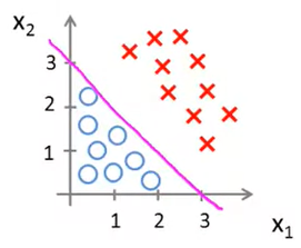
If we try to plot the above equation we will get something like this :

So according to this plot everything to right of this line will be “ y = 1 “ since X₁ + X₂ >= 3. Similarly, everything to left of this line will be “ y = 0 “ since X₁ + X₂ < 3. This line is called decision boundary. This line seperates the region of y=1 and y=0.

Non-linear Decision Boundary

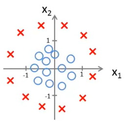
Now their might be some cases where the plot is not simple as it was in previous section. Lets take another example, see this plot :

As you can imagine in the above plot no straight line can create a decision boundary. That means no straight line can differenciate between y=1 and y=0. So how are we going to handle this scenerio? To find these non-linear decision boundary we will require a higher order equation. Something like :

h(x) = g(θ₀ + θ₁X₁ + θ₂X₂ + θ₃X₁² + θ₄X₂²)

As we assumed some values of θ in previous example, lets imagine some values again for this case :

θ₀ = -1
θ₁ = 0
θ₂ = 0
θ₃ = 1
θ₄ = 1

After substituting

h(x) = g(-1 + X₁² + X₂²)

So for prediction :

1. y = 1 : if -1 + X₁² + X₂² >= 0 => X₁² + X₂² >= 1
2. y = 0 : if -1 + X₁² + X₂² < 0 => X₁² + X₂² < 1

If you can relate, this is an equation for a circle. So it will draw a circle and whatever is inside the circle will have y=0 and whatever is outside the circle will have y=1. And this way we created decision boundary for non-linear equations. Similarly if we increase the degree of hypothesis function we can create even more complex decision boundaries.